
It is possible that on some occasion you have opened an Excel document and you have found that a drop-down list opens in some of its cells. This is a very handy feature of Microsoft spreadsheets that you can use too. In this post we explain how to create drop down list in excel
This is a very useful function, especially when we are working with sheets and templates in which the same options are repeated. But in addition to being practical, it is also a very visual resource that gives a more professional look to any document.
The drop-down lists (in English, down drop list) allow users of Excel select an item from a predefined list. It is a particularly suitable resource for making forms, because thanks to it the data entry is faster and also more precise.
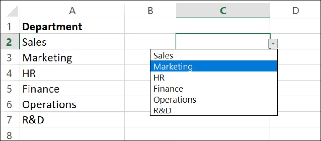
How do these lists work? When we select a cell which contains a list, we will see next to it the icon of a small arrow. When clicking on it, this list is displayed with a series of options among which we have to select one.
The basic idea of creating dropdown lists in Excel is to provide the user with a limited number of options. In addition, the introduction of data with errors or misspellings is avoided.
Create a drop-down list in Excel step by step
These are the steps to follow to create drop-down lists in Excel:
Step 1: Select the cell
If we already have an Excel sheet that is more or less organized and structured and we consider the question of inserting one or more drop-down lists in it, the first thing we must do is select with the mouse pointer the cell or cells in which we want the list to open when we click on it.
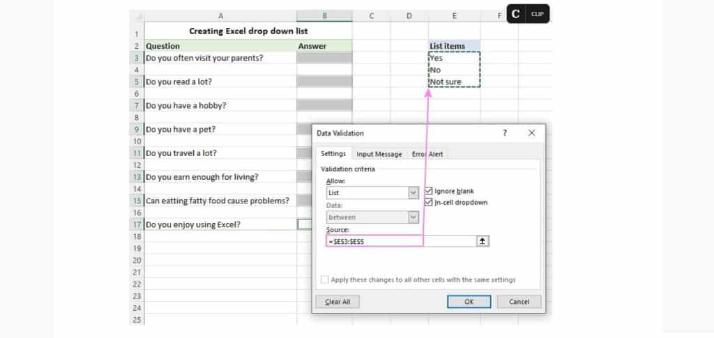
Step 2: Data validation
Next, we click on the “Data” tab. Once open, we go to the "Data Tools" group where we must find and press the option "Data validation". Depending on the version of Excel that we have installed, the icon may vary, although in general it usually looks like two cells, one validated and the other not.
Step 3: Select and configure the list
After validation, a drop-down list opens, in which we choose the option "Ready". There we also have other options through which we will be able to limit the content of the cell to certain formats (numbers, dates, hours, etc.). Then, we can proceed in two different ways:
- write the elements that we want to offer as options within the list (they must be separated by a comma, without spaces).
- Select a range of cells that contain those options and validate it by clicking on the arrow icon next to the cell where the drop-down list will open.
Once the process is complete, we will see how clicking on the chosen cell will display the list that we have configured. If we want to repeat the operation in another cell of the document, it will be enough to copy it to the clipboard and paste it in the new cell.
Create a dynamic dropdown list in Excel
If we plan to regularly change the items in our dropdown list in Excel, it may be more appropriate to choose to create a dynamic dropdown list. This is a variant of what we have seen in the previous section, with the particularity that, in this case, every time we make a change in the cells or in the source list, the drop-down list will be updated automatically.
There are two ways to create this type of list: with the same method that we have explained before or using a regular named range and referencing it with the OFFSET formula. We explain how it is done below:
- First we need to write the dropdown menu items in separate cells.
- Then we create a named formula (to do this, use the Control + F3 key combination to open the dialog).
- Once the new name is written in the "Name" box, we introduce the following formula:
=OFFSET(Sheet!$A$2, 0, 0, COUNTA(Sheet3!$A:$A), 1) *
Sheet: name of the sheet.
A : The column where the dropdown items are located.
$A$2: The cell that contains the first item.
When we already have the formula defined, we only have to create a drop-down menu based on a range of cells, as we have seen in the previous section. The setup process is a little more laborious, but it will be worth it if we have to work with a constantly changing list of source cells.
(*) As can be seen, this formula consists of two functions: OFFSET and COUNTA. The second is to count all non-blank cells in the referenced column. This count is used in turn by the OFFSET function.