
Conditional formatting in Excel is an option that can help us digest the information that a spreadsheet raises in a much more friendly way.. Excel documents are often full of calculations and figures that will be seen or analyzed by yourself or others, so it would be great to have an alternative that allows us to speed up this process. The Microsoft tool has been characterized by incorporating dozens of functions that allow anything from being done faster to automating it. Therefore, today we are going to show you everything you need to know to start using the conditional format in your work.
In this way, you will be able to enhance the usefulness of your Excel table and also save a lot of time in tasks of highlighting information and analysis.
What is conditional formatting in Excel?
Excel is a program full of tools that not only cover the area of calculations, but also what refers to the format and the way in which the data and information is presented on the sheet.. The latter is essential, considering that Excel workbooks are not usually kept for their own consumption, but are generally sent to other people for review and analysis. While doing the latter, it is common for certain figures to be highlighted depending on the factors being observed, however this also opens the door for human error. We could easily miss an important cell or highlight one that doesn't meet what we're looking for.
To eliminate this problem, the conditional format appears in Excel, which, as its name indicates, allows us to format a cell or range of cells, according to the fulfillment of a specific condition.. For example, if the minimum sales goal for your business is €500, mark the cells whose figures do not reach this number in red. This way, the Excel sheet will speak for itself through this formatting code that you set for the key fields.
The uses that you can give to this function are multiple and as we mentioned before, it will give a much greater utility to the spreadsheet. Continuing with the sales example, if you add up each transaction of the day and apply a conditional format to the cell that shows the total, it will change color just when you reach the minimum goal. This serves as a rather attractive visual indicator for a simple Excel document.
Elements of conditional formatting
The conditional format area in Excel is very wide and it is worth knowing it to take advantage of the options that it incorporates and that give us the possibility of giving life to our spreadsheet. However, we can say that its use is really simple and it is enough to know its three main components to become fully familiar with it. These are: the conditions, the rules and the formats.
Terms of use
A condition is nothing more than the factor that we use as a reference to define if something will happen or not.. For example, if it rains, then I will take an umbrella, which means that taking the umbrella has the conditional that it rains. The same happens in Excel with the conditional format, a condition is established based on whether a cell has a certain number, text or date and if so, a rule will be applied.
Rules
The rules are those that establish what will happen if the previously stated condition is met.. Continuing with the example of the umbrella, the rule in this case is to take it with you, if it rains. In this sense, if we take it to Excel, the rule will indicate the format that will be applied to the rule when the condition is met.
Formats
Within the Microsoft office suite, the formats represent everything related to the aesthetic and visual section of the document in which we work. This goes from the font, to its size, color and background color, so conditional formatting is nothing more than a tool that allows you to apply all this, based on the conditions and rules that we explained before.
How to use conditional formatting in Excel?
Steps to apply basic conditional formatting
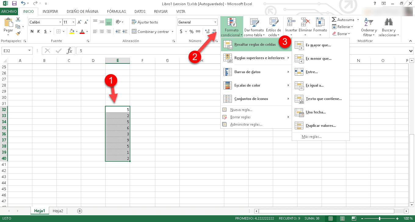
If you already have an idea to apply conditional formatting in your Excel sheet, you should know that doing so is quite simple. To get started, we must first select the cell or range of cells that we want to format according to a condition. Then click on «Conditional format» and then go to «Cell Rules“, which will display a whole series of options that you can apply. These range from identifying greater, lesser or equal values, to texts and dates.
By clicking, for example, on «Older than", a small popup window with two fields will be displayed. In the first, you will have to enter the reference figure and in the second you will be able to choose between several predefined formats or add a custom one.
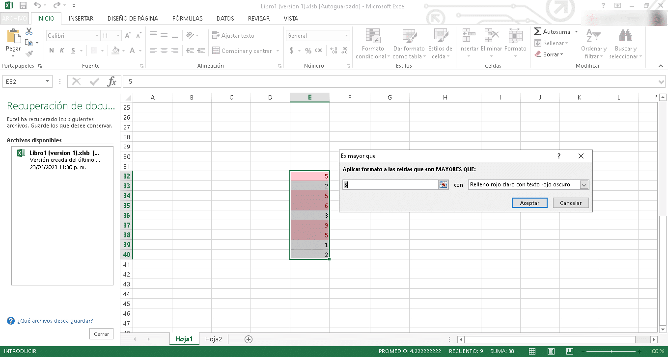
Finally, click on «Accept» and that's it, now the numbers that are greater than the one you previously indicated will be marked with the selected format.
Conditional Formatting with Icons
It is worth noting that conditional formatting not only works by changing the fill color of cells and characters, it is also possible to display icons instead of the classic colors. This is very interesting because it increases the communicative and analytical potential of the Excel sheet, making it much easier to recognize what is happening with each element.
To use this type of conditional formatting, we'll start by selecting the cell or cell format you want to format. Then click on «Conditional format«, go to the rules section and select what you want to set the condition to be met.
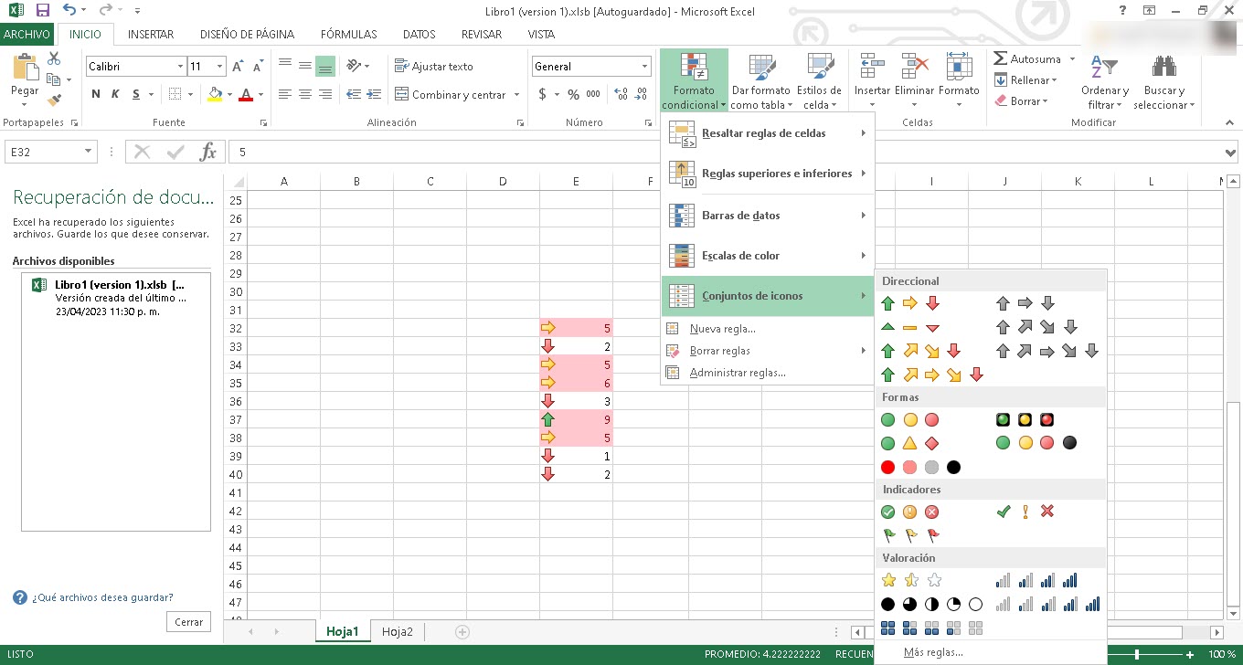
Then click again on "Conditional format» but, this time go to «icon set» and then select the one you want.
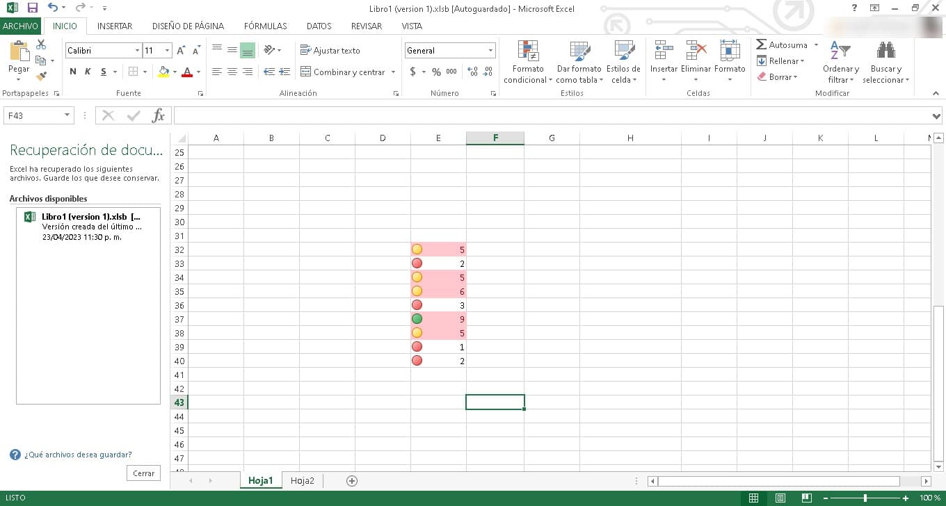
Immediately, you will see how they appear on the left end of each cell with the color that identifies them.
Conditional Formatting with Data Bar
In the same way that we use icons or colors for cells, we can also work with data bars. This is especially useful if we are generating figures that need to be compared with others. The data bars will allow us to have a much clearer visual approach to this comparison, making the information more accessible.
If you want to work with data bars in Excel's conditional formatting, you must follow the same steps that we discussed above. That is, select the cell or range of cells, click on «Conditional format» and select the rule you want to apply from the Rules menu. Then, repeat the process by going to “Conditional format» and then enter «data bars» to choose the type of bar you want to add. When you click it, they will already have been added to your spreadsheet.
As we can see, conditional formatting is a real wonder that will enhance your spreadsheet, your use of Excel, and the task of highlighting data and doing analysis. It is a really easy option to use, so it is worth trying it in any of your Excel workbooks.