
Microsoft Excel spreadsheets are an essential program for millions of people. Especially in the professional field, they are a program that is used daily, so it is very important for many users. In these cases, when working with the program, there may be people who have to work with a lot of data, but it is not always comfortable to have the full screen in the spreadsheets.
Luckily, there is an option that can help a lot the work Microsoft Excel. Since the program allows us to divide the screen, which is something that will allow us to work better with these spreadsheets at all times. Especially if the screen is not too large, so that we do not see all the data.
Over the years, they have been introduced performance improvements in Microsoft Excel. This is something that has allowed users to make better use of the program, as well as having additional functions, which allow its use in all kinds of situations. Although, as we already know, on many occasions we work with huge amounts of data, which occupy many rows and columns. Which makes the handling not entirely comfortable.
In these cases, we can slightly customize the interface in the program. A simple trick, but very helpful to work better at all times. In this way, if you have to work with a lot of data using this program on your computer, you will be able to do it in the best possible way. So you don't make mistakes when having to work with a high volume of data.
Split screen in Microsoft Excel
Microsoft Excel introduced the divide function a few years ago, which as its name suggests, allows us to divide the screen in a better way. Since what it does is to be able to handle these cells in a way that is faster and more effective for the users. Since the contents will be displayed in several areas, we can divide into two or four dimensions, which we can customize. Thus, depending on what we need at all times, we can divide said screen in the best way.
If we have a screen with a lot of data, we can see it in a better way or access it, having it all on one screen at the same time. It avoids us having to move through said spreadsheet, which is very tiring or causes us to skip any data that we want to see. For this, we have to open the spreadsheet that we want in Microsoft Excel on our computer. Then we can start.
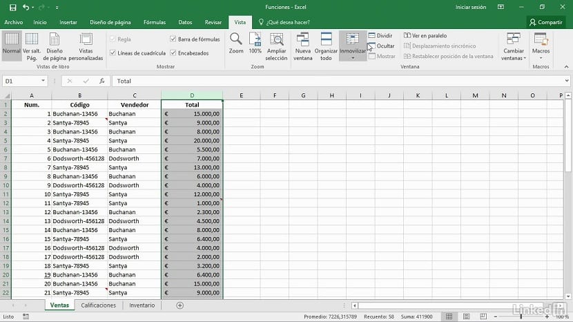
The first thing we have to do is place the cursor in the first square of the sheet, in A1. Then, we go to the top menu of the program, where we have to click on the View section. Next, several options will be shown in this section. One of the options that we find in it is to Divide. This is the option we have to click on in this case. By doing this, the spreadsheet is divided into four equal grids on the screen, where we have all the data from it. If we want, we can move the grid, which we can resize to our liking, so that it better suits the use we have to do. We can use two grids if we think it is better in this regard.
Microsoft Excel gives us quite a few options in this regard. Since we can divide the screen horizontally, but also vertically, it depends on what each one needs. But we can use this function of dividing in a way that is more comfortable depending on the document, screen or the amount of data that there is. So it is a feature that we can customize quite easily in the program. So it is a good option to use at all times.